In this tutorial, we 'll first take a look at the Youtube API to retrieve comments data about the channel as well as basic information about the likes count and view count of the videos. Then, we will use Nltk to see most frequently used words in the comments and plot some sentiment graphs.
The Data
With the script below, we first query the video channels providing the channel ID then for every video we get a list of comments (Youtube limits this number to 20 comments per query)
from apiclient.discovery import build
import pandas as pd
import time

DEVELOPER_KEY = ""
YOUTUBE_API_SERVICE_NAME = ""
YOUTUBE_API_VERSION = ""

youtube = build(YOUTUBE_API_SERVICE_NAME, YOUTUBE_API_VERSION, developerKey=DEVELOPER_KEY)

def get_videos_FromChanel(youtube, channelId,order):
    search_response = youtube.search().list(
        channelId=channelId,
        type="video",
        part="id,snippet",
        maxResults=50,
        order=order
    ).execute()

    return search_response.get("items", [])

def get_comment_threads(youtube, videos):
    tempComments = []
    for video in videos:
        time.sleep(1.0)
        print video["snippet"]["title"]
        results = youtube.commentThreads().list(
            part="snippet",
            videoId=video["id"]["videoId"],
            textFormat="plainText",
            maxResults=20,
            order='relevance'
        ).execute()


        for item in results["items"]:
            comment = item["snippet"]["topLevelComment"]
            tempComment = dict(videoId=video["id"]["videoId"], videoName=video["snippet"]["title"],nbrReplies = item["snippet"]["totalReplyCount"],author = comment["snippet"]["authorDisplayName"],likes = comment["snippet"]["likeCount"],publishedAt=comment["snippet"]["publishedAt"],text = comment["snippet"]["textDisplay"].encode('utf-8').strip())
            tempComments.append(tempComment)

    return tempComments
then you can call the function using :
videos = get_videos_FromChanel(youtube, "CHANNEL_ID","viewCount")
Statistics
Youtube has a special option to retreive the statistic data, we just have to query the video list method using the "statistic" option.
def getVideoInfos(videos):
    videoList = {}
    for search_result in videos:
         if search_result["id"]["kind"] == "youtube#video":
             videoList[search_result["id"]["videoId"]] = search_result["snippet"]["title"]

    s = ','.join(videoList.keys())
    videos_list_response = youtube.videos().list(id=s,part='id,statistics').execute()
    res = []
    for i in videos_list_response['items']:
         temp_res = dict(v_title = videoList[i['id']])
         temp_res.update(i['statistics'])
         res.append(temp_res)

    data = pd.DataFrame.from_dict(res)
    data['viewCount'] = data['viewCount'].map(lambda x : float(x))
    data['commentCount'] = data['commentCount'].map(lambda x : float(x))
    return data

data = getVideoInfos(videos)

infos.sort('viewCount',ascending=0).head(20).plot(kind='bar', x='v_title',y='viewCount')
This is what I get for the view count of the shots of
Awe videos
channel:

We can have the same plots for likes counts and comments count, and plot scatter plots to see if there is a correlation between these features.
We can note that the third video has only been uploaded for a few days at the time I’m writing this article, that's what we call a buzz video.
An interesting chart to plot would be the number of views/time online.
Comments analysis
-
Word Frequency
What do people talk about in the comments ? What do they like/hate the
most about the channel ?
In order to answer these questions we can look at the word frequency in
the comments. We can use the "nltk" package to see the distribution :
import nltk
from nltk.probability import *
from nltk.corpus import stopwords
import pandas as pd

all = pd.read_json("comments.csv")

stop_eng = stopwords.words('english')
customstopwords =[]

tokens = []
sentences = []
tokenizedSentences =[]
for txt in all.text:
    sentences.append(txt.lower())
    tokenized = [t.lower().encode('utf-8').strip(":,.!?") for t in txt.split()]
    tokens.extend(tokenized)
    tokenizedSentences.append(tokenized)

hashtags = [w for w in tokens if w.startswith('#')]
ghashtags = [w for w in tokens if w.startswith('+')]
mentions = [w for w in tokens if w.startswith('@')]
links = [w for w in tokens if w.startswith('http') or w.startswith('www')]
filtered_tokens = [w for w in tokens if not w in stop_eng and not w in customstopwords and w.isalpha() and not len(w)<3 and not w in hashtags and not w in ghashtags and not w in links and not w in mentions]

fd = FreqDist(filtered_tokens)
FreqDist returns a list of tuples containing each word and the number of its occurences. Let"s plot a bar chart to visualize it:
import scipy
import pylab
import operator
from operator import itemgetter, attrgetter

sortedTuples = sorted(fd.items(), key=operator.itemgetter(1), reverse=True)
a = [i[0] for i in sorted_x[0:20]]
b = [i[1] for i in sorted_x[0:20]]

x = scipy.arange(len(b))
y = scipy.array(b)
f = pylab.figure()
ax = f.add_axes([0.5, 0.5, 1.5, 1.5])
ax.bar(x, y, align='center')
ax.set_xticks(x)
ax.set_xticklabels(a)
f.show()
And the result :
The most used words are "love" (141 occurrences), "like" (89 occurrences) then "think" and "life". Pretty deep !
-
Sentiment Analysis
In order to analyze the comments sentiments, we are going to train a Naive Bayes Classifier using a dataset provided by nltk. This could be imroved using a better training dataset for comments or tweets.
The reviews are classified as "negative" or "positive", and our classifier will return the probability of each label. We will compute a score = prob("positive") - prob("negative") to get a score between -1 an 1.
Training the classifier
import pandas as pd
import nltk.classify.util
from nltk.classify import NaiveBayesClassifier
from nltk.corpus import movie_reviews

###############
def word_feats(words):
    return dict([(word, True) for word in words])
###############

negids = movie_reviews.fileids('neg')
posids = movie_reviews.fileids('pos')

negfeats = [(word_feats(movie_reviews.words(fileids=[f])), 'neg') for f in negids]
posfeats = [(word_feats(movie_reviews.words(fileids=[f])), 'pos') for f in posids]

trainfeats = negfeats + posfeats

classifier = NaiveBayesClassifier.train(trainfeats)
###############

all = pd.read_json("comments.csv")

all['tokenized'] = all['text'].apply(lambda x: [t.lower().encode('utf-8').strip(":,.!?") for t in x.split()] )
all['sentiment'] = all['tokenized'].apply(lambda x: classifier.prob_classify(word_feats(x)).prob('pos') - classifier.prob_classify(word_feats(x)).prob('neg') )
Once the classifier trained, we added a column with the sentiment score using the "classifier.prob_classify" function.
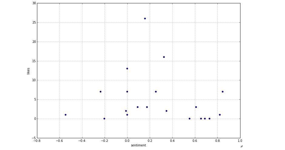
Let's see the results for the first video in a scatter plot (versus likes)
videos = all.videoId.unique()
all[all.videoId==videos[1]].plot(kind='scatter', x='sentiment', y='likes', figsize=(12,8))
For the next one,
A cool thing to do here is to see what's the text of every comment. The best thing to do is to have an interactive plot where hovering on a point shows the comment text. This could be done with the d3.js library. We can also make the axis interactive and add animations to animate the points when for example changing the sentiment axis to the publishing date of the comment...
Next Steps:
- Adding a plot for "number of views"/"time online"
- Interactive d3.js plot to see the comment text when hovering on he comment.


